Genetic
algorithms (GA) have become a popular optimization method as they often succeed
in finding the best optimum in contrast to most common optimization algorithms.
Genetic algorithms imitate the natural selection process in biological evolution
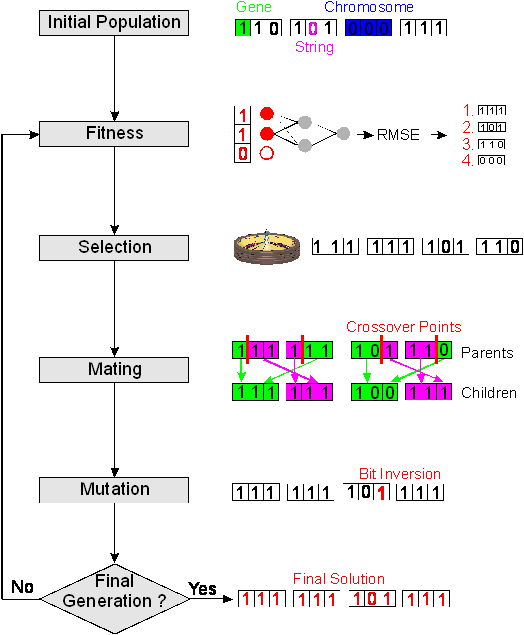
with selection, mating reproduction and mutation. On the left-hand side of figure
5, the sequence of the different operations of a genetic algorithm is shown.
The parameters
to be optimized are represented by a chromosome whereby each parameter is encoded
in a binary string called gene. Thus, a chromosome consists of as many genes
as parameters to be optimized. A population, which consists of a given number
of chromosomes, is initially created by randomly assigning "1" and
"0" to all genes. On the top right part of figure
5, the different terms are graphically shown for a population of 4 chromosomes
with 4 genes (in the case of variable selection a gene contains only a single
bit string for the presence and absence of a variable). The best chromosomes
have the highest probability to survive evaluated by a so-called fitness function.
The next generation is reproduced by selecting the best chromosomes, mating
the chromosomes to produce an offspring population and by an occasional mutation.
The evaluation and reproduction steps are repeated until a certain number of
generations, until a defined fitness or until a convergence criterion of the
population are reached. In the ideal case, all chromosomes of the last generation
have the same genes representing the optimal solution. The theory and benefits
of GA in variable selection have been described several times in literature
[98]-[103] and will not be repeated
here, as there are uncountable variants of the different genetic operators.
Instead, a description of the GA implementation, which has been used in this
work and its special features like the implementation of the fitness function
and the other genetic operators will be further discussed and are illustrated
on the right side of figure 5.
figure 5: Flow chart of a genetic
algorithm (left side) and explanations of the different operations by the application
of the genetic algorithm to a variable selection problem with 3 variables and
neural networks for the evaluation of the fitness.
In
this work, the initial population of the GA is randomly generated except of one
chromosome, which was set to use all variables. The binary string of the
chromosomes has the same size as variables to select from whereby the presence
of a variable is coded as "1" and the absence of a variable as "0".
Consequently, the binary string of a gene consists of only one single bit.
After evolving the fitness of the population, the individuals are selected by
means of the roulette wheel. Thereby, the chromosomes are allocated space on a
roulette wheel proportional to their fitness and thus the fittest individuals
are more likely selected. In the following mating step, offspring chromosomes
are created by a crossover technique. A so-called one-point crossover technique
is employed, which randomly selects a crossover point within the chromosome.
Then two parent chromosomes are interchanged at this point to produce two new
offspring. After that, the chromosomes are mutated with a probability of 0.005
per gene by randomly changing genes from "0" to "1" and
vice versa. The mutation prevents the GA from converging too quickly in a small
area of the search space.
A crucial
point in using GA is the design of the fitness function, which determines what
a GA should optimize. In the case of a variable selection for calibration, the
goal is to find a small subset of variables, which are most significant for
a regression. In this work, the calibration is based on neural networks for
modeling the relationship between the input variables (many time-dependent sensor
signals) and the responses (concentrations of the different analytes). Thus,
the evaluation of the fitness starts with the encoding of the chromosomes into
neural networks whereby "1" indicates that a specific variable is
used and "0" that a variable is not used by the network. Then the
networks are trained with a calibration data set and after that, a test data
set is predicted. Finally, the fitness is calculated by a so-called fitness
function f. In contrast to many
GA for variable selection found in literature [99],[101],[129]-[131],[243],
the fitness function used for the GA variable selections in this work takes
into account not only the prediction error of test data but also partially the
calibration error and primarily the number of variables used to build the corresponding
neural nets:
(16)
Thereby
nv is the number of
variables used by the neural networks, ntot
is the total number of variables and MRMSE is the mean root mean square error
of the calibration respectively test data. The MRMSE is defined in equation
(17) with N
as total number of samples predicted, M as total number of analytes, as predicted concentration
of analyte j in sample i
and as the corresponding
known true concentration:
(17)
The fitness
function can be broken up into three parts. The first
two parts correspond to the accuracy of the neural networks. Thereby MRMSEcal
is based on the prediction of the calibration data used to build the neural
nets, whereas MRMSEtest is based on the prediction of separate test
data not used for training the neural networks. It was demonstrated in [11]
that using the same data for the variable selection and for the model calibration
introduces a bias. Thus, variables are selected based on data poorly representing
the true relationship. On the other hand, it was also shown [11],[132]
that a variable selection based on a small data set is unlikely to find an optimal
subset of variables. Therefore, a ratio of 1:4 between the influence of calibration
and test data was chosen. Although being partly arbitrary this ratio should
give as little influence to the calibration data as to bias the feature selection
yet taking the samples of the larger calibration set partly into account. The
third part of the fitness function rewards small networks using only few variables
by an amount proportional to the parameter a.
The choice of a influences the number of variables used by the evolved
neural nets. A high value of aresults in only
few variables selected for each GA whereas a small value of a
results in more variables being selected.
As the
initial weights of a neural network are randomly set, the network finds another
local minimum of the error surface for each calibration run with a slightly
different performance of prediction. In order to reduce the variance of the
error of prediction due to random weight initialization the fitness is averaged
in expression (17) over 20 training
and prediction sessions per network topology (evaluation of 20 parallel neural
networks with different initial weights).